4. Data preprocessing and constructing databases for fast routing

Accessibility computations are based on repeating computations of the car and transit fastest routes between buildings. These computations demand topologically clean layers of roads and buildings, and the user’s layers are tested and if necessary corrected in the Data preprocessing section of the Accessibility Calculator menu. The layers necessary for visualization of the accessibility calculations are also constructed at this stage. 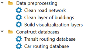Then, to save computation time, the networks that are necessary for accessibility computations are stored as two databases, one for transit and one for car network routing. The data must be cleaned, and the databases must be constructed at the beginning of the accessibility study. Each version of the transit or road network demands a separate database that is stored in a dedicated folder. It is worth constructing the dataset for a large area (of up to a million buildings) that covers all potentially interesting locations and regions. The menu for data preprocessing and database construction consists of two sections (Figure 1)

Figure 1. Data processing section of the Accessibility Calculator menu

In this tutorial, we construct topologically correct versions of the road network and buildings and then exploit them to construct three databases – one for computing car accessibility and two for computing transit accessibility for two different versions of the transit networks. We limit our examples to the Tel Aviv Metropolitan Area (TAMA), with its 250K buildings, and construct the car routing database for this area only. The databases for transit routing are constructed for the entire Israel. Specifically, we use

The gis_osm_roads_free OSM TAMA road layer, August 2024.
The gis_osm_buildings_a_free OSM buildings layers for TAMA, August 2024.
Two versions of the GTFS databases, one for June, 2018, reflecting the state of the transit system before the Red LRT line was established in the Tel Aviv Metropolitan area and one for June, 2024, after the Red LRT line started to function. Each GTFS dataset contains``stops.txt``, stop_times.txt, routes.txt, trips.txt and calendar.txt.

It is recommended to open the layers of buildings and roads in your QGIS project before cleaning them and to validate that these are indeed the layers you plan to work with. The path to the GTFS dataset must be provided as a parameter of the construction procedure. The clean layers of roads and buildings, as well as the layers built for visualization, will be added to your QGIS project.

4.1. Topological cleaning of the road and building layers

The GIS layers of roads and buildings can be topologically inconsistent. There are many types of topological errors and the most frequent for the road network is the lack of a junction at an intersection of two visually overlapping links or two or more links that remain unconnected at a junction. In the case of the layer of buildings, the most frequent error is overlapping building foundations. Accessibility computations demand road and transit routing and, thus, cannot be performed with the topologically inconsistent road layers. To be sure that the spatial data that we use is correct for accessibility computation we have included the basic topological cleaning procedures into the plugin. If the layers of roads and buildings are topologically correct, the cleaning procedures will not change them. Cleaning road network The Accessibility Calculator is performed with the v.clean GRASS procedure, see details at https://grass.osgeo.org/grass-stable/manuals/v.clean.html. It is done in three steps. First, the links’ ends are snapped at junctions. This is done by applying v.clean.snap with the threshold of 1 m. That is, all links’ ends that are at a distance of 1 m or less form from each other will be snapped to one of them. In the second step, v.clean.break is employed - the intersecting links are broken at the points of intersection, and new junctions are created at these points. Then v.clean.rmdupl is employed to reveal the overlapping links and the additional postprocessing is performed to preserve one of them only.

Note

The OSM layer of roads contains significant topological errors and the cleaning procedures that we employ in the Accessibility Calculator make the layer formally topologically consistent. However, it may happen that, contextually, the layer of roads does not reflect the real structure of the road network. One of the ways to test this is to employ the v.clean procedure, in the order and with the parameters we mention above, manually. You can also vary the 1m threshold that we employ. When cleaning procedures are applied manually, the results, at each step, include the errors report that will help you to understand the road layer inconsistencies. Then you could decide whether to edit the roads layer or keep it as is.

To perform data cleaning for roads choose the Data preprocessing → Clean road network and enter the parameters (Figure 2):

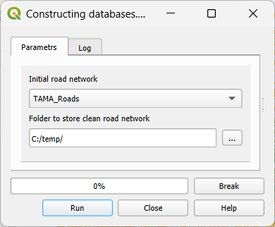
Figure 2. Clean road network dialog

Initial road network - the initial layer of roads. We advise opening the layer in the current QGIS project and to ensure that the choice of the layer is correct.
Folder to store clean road network - the folder to store the clean road layer.

The cleaning of the layer of buildings is performed in several steps. In the first step, the delete holes algorithm is employed to delete holes in the buildings, see https://docs.qgis.org/3.34/en/docs/user_manual/processing_algs/qgis/vectorgeometry.html#qgisdeleteholes. Then, the features with the absent (NULL) geometry are deleted from the layer and multipart features are split into single parts https://docs.qgis.org/3.34/en/docs/user_manual/processing_algs/qgis/vectorgeometry.html#qgismultiparttosingleparts. Finally, the building features that have got identical identifiers are selected and their identifiers are made unique by adding “_1,” “_2,” etc. to the repeating identifier. To perform cleaning of the layer of buildings choose the Data preprocessing → Clean road network option, and enter the parameters (Figure 3):

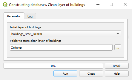
Figure 3. Clean layer of buildings dialog

Initial layer of buildings - the initial layer of roads. We advise to open the layer in the current QGIS project and to ensure that the choice of the layer is correct.
Folder to store clean layer of buildings - the folder to store the clean buildings layer.

After setting the parameters of each of the cleaning procedures, click Run to start. The Progress bar will show the progress of the computations. If something went wrong, you could break the process of dictionary construction by pressing Break. The Log tab contains information about the parameters, information on the process of construction, and the edits that were performed. The clean layer of roads and buildings will be added to the current GIS project. For the example of cleaning the road network and buildings layer of TAMA see section 10.2.

4.2. Building layers for visualization

Accessibility Calculator assesses accessibility at resolution of a single building and in every computation, each accessible building is assigned a computed measure of accessibility. The results of computations are thus visualized using the thematic maps at the resolution of buildings or lower. First, the results can be visualized with the buildings themselves. However, a lion’s share of the constructed area is not covered by the buildings and these maps are inconvenient to use. The coverage becomes continuous if buildings are substituted by their Voronoi polygons. The coverage of the buildings’ Voronoi polygons is built based on the building centroids, applying https://docs.qgis.org/3.34/en/docs/user_manual/processing_algs/qgis/vectorgeometry.html#qgisvoronoipolygons algorithm, with polygons’ identifiers repeating identifiers of the buildings. Then the buffers of buildings’ centroids of 50m radius are constructed and the layer of the Voronoi polygons is overlapped with the layer of buffers to avoid too large Voronoi polygons that are always constructed at the boundary of the constructed area. The buildings’ Voronoi polygons have different sizes and can be small, 10 or less meters in diameter. To allow uniform coverage of the built area, the Accessibility Calculator, in addition to constructing the layer of Voronoi polygons of buildings, constructs four layers of hexagons of 100, 200, 400, and 800 m sides. Each layer covers the entire extent of the layer of buildings layer. The hexagon layers are constructed applying the https://docs.qgis.org/3.34/en/docs/user_manual/processing_algs/qgis/vectorcreation.html#qgiscreategrid algorithm. Then, the hexagons that do not overlap any building are deleted from each layer and each hexagon is assigned the identifier of the building that is closest to the hexagon’s centroid. If several buildings are at the same distance from the centroid, the minimal identifier is chosen. The same building may be closest to more than one hexagon’s centroids. At the last stage of construction of the layers for visualization, these hexagons are dissolved into one. To build layers for visualization choose the Data preprocessing → Build visualization layers option, and enter the parameters (Figure 4):

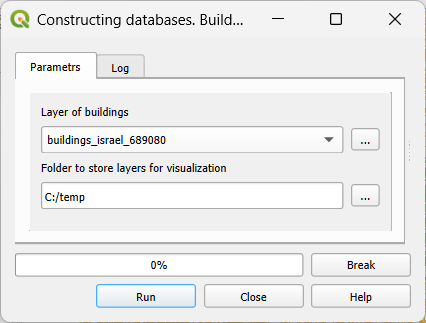
Figure 4. Build layers for visualization dialog

Layer of buildings - the initial layer of buildings. We advise opening the layer in the current QGIS project and to ensure that the choice of the layer is correct.
Folder to store layers for visualization - the folder to store the layers for visualization.

After setting the parameters of each of the cleaning procedures, click Run to start. The Progress bar will show the progress of the computations. If something went wrong, you could break the process of dictionary construction by pressing Break. The Log tab contains information about parameters and the process of construction. Five layers – one of the Voronoi polygons, and four layers of hexagons will be constructed. These layers will be automatically added to the current GIS project. Yet we recommend opening them to check that they reflect your expectations and properly match the layer of buildings. For the example of cleaning the road network and buildings layer of TAMA see section 10.2.

4.3. Building database for transit accessibility

After the layers of roads and buildings are cleaned, we can build the databases for accessibility computations. At this stage, the data on roads, buildings, and public transport data are translated into a special database format that allows fast data retrieval for accessibility computations. In addition to this transformation, the buildings that are not connected to the road network are connected to the nearest road link. In this way, we become able to estimate the length of the walk to the bus stops around the chosen location. To build the database for transit routing choose the Construct databases → Transit routing database option. In the dictionary construction dialog (Figure 5), enter the parameters:

Figure 5. The Transit routing database construction dialog

Roads database folder - the folder of the roads database.
Layer of buildings - the layer of buildings. Must be open in a current GIS project.
id - the unique identifier of a building.
GTFS folder - the path to the folder that must contain all necessary GTFS files: stops.txt, stop_times.txt, routes.txt, trips.txt, calendar.txt.
Folder to store transit database- the folder to store the transit routing database.

Click Run to start. The Progressbar will show the progress of the computations. If something went wrong, you could break the process by pressing Break. The Log tab contains information about the parameters and the process of construction. For a detailed example of building a transit routing database for TAMA see section 10.2.

4.4. Building database for car routing

Choose the Data preprocessing → Car routing database. Note that the database construction demands two tables (the right part of the dialog). Their meaning is explained in the next section 4.5. In the dialog (Figure 6), enter the parameters:

Figure 6: Car routing database construction dialog

Roads database folder — the folder of the roads database.
link type — the field of the link’s type in the layer of roads.
direction — the field of traffic direction in the layer of roads.
speed — the field of the link’s speed in the layer of roads.

Currently, we presume that the direction field contains the OSM traffic direction codes:
B: Two-way link,
F: One-way link, the driving is allowed along the direction the link is drawn,
T: One-way link, driving is allowed against the direction the link is drawn.

Layer of buildings - the layer of buildings, must be opened in a current GIS project.
id - the unique identifier of a building.
Default speed (km/h)- the link’s speed in case the link’s type is missing in the table of links’ speeds.
Folder to store car database - the folder to store the database for car routing.

Click Run to start. The Progress bar will show the progress of the computations. If something went wrong, you could break the process by pressing Break. The Log tab contains information about the parameters and the process of construction. For a detailed example of building a database for car routing in TAMA see section 10.2.

4.5. Car Speed and Congestion Delay Index

To compute car accessibility, one must know traffic speed along the route. In the current version of the plugin, the traffic speed is defined by the type of road - a highway, major city street, neighborhood secondary street, etc., and the hour of the day. The necessary parameters are stored in two tables that are located in the plugin folder and can be edited. The free-flow traffic speed V_p, by the road link types p, is given in the car_speed_by_link_type.csv table (Figure 7, left). This table contains three fields.
seq — the sequential number of the row,
link_type — the OSM type of a link, and
speed — the car speed on the link of this type. The OSM road layer may contain links whose type is missing in the car_speed_by_link_type.csv table. For these links, the Default speed (km/h) will be used. The hour of the day is reflected by the Congestion Delay Index (CDI) - a ratio of the average, for the hour of a day, speed, to the free flow speed. The CDI values, by hours, are given in the cdi_index.csv table (Figure 7, right). The speed V_p(t) on the link of a type p at the hour t is calculated as V_p(t) = V_p*CDI_t

link type	speed (km/h)
busway	18
cycleway	15
footway	3
motorway_link	40
track	40
residential	30
service	40
secondary	50
living_street	30
tertiary_link	50

hour	CDI
0	1.0
1	1.0
2	1.0
3	1.0
4	1.0
5	0.9
6	0.75
7	0.6
8	0.6
9	0.65

Figure 7. Several first rows of the free flow speeds table car_speed_by_link_type.csv (left) and the CDI table cdi_index.csv (right). The values of the free flow speed and CDI can be changed by the user.